3 Regression
Perform a regression analysis on MODIS Normalized Difference Vegetation Index to observe the spatial distribution of greening and drying over the last two decades.
3.1 Settings and data
Set some time settings and load the required data. The filter options allow you to filter on specific years and months as specified by the user in the time settings. You can play around with the time settings. For example, alter these settings such that you acquire NDVI trends for the summer period for the years 2010 to 2015.
// time settings
var yearrange  = [2000,2017];   // limit calculations to specific range of years
var monthrange = [1,12];        // limit calculations to specific range of months

// load MODIS NDVI collection
var ndvi = ee.ImageCollection("MODIS/006/MOD13A1");

// Filter collection
ndvi = ndvi.filterDate(yearrange[0]+'-01-01',yearrange[1]+'-12-31')
           .filter(ee.Filter.calendarRange(monthrange[0],monthrange[1], 'month'))
           .select('NDVI')
A scaling factor is applied to the original data in the catalog (0.0001). To get the correct NDVI value, this factor first must be applied to each image in the filtered collection with the code below. Type “MODIS/006/MOD13A1” in the search bar, select the top result and look at the band descriptions of this dataset where the scaling factors are defined.
Most image properties are lost when you apply reducers or arithmetic functions to images. To retain the time information that is stored with each image the system:time_start property is transferred using the set and get functions.
3.2 Derive annual composites
Annual mean NDVI images can be produced with the following code. It loops over a list of years, applies a time filter to the image collection in each loop, calculates a mean composite, and adds the current year as a constant image band.
// Perform temporal reduction to get yearly mean NDVI images
var years   = ee.List.sequence(yearrange[0],yearrange[1]);
var yearmeans = ee.ImageCollection.fromImages(
    years.map(function (yr){
      return ndvi.filterDate(ee.Date.fromYMD(yr,1,1),ee.Date.fromYMD(yr,12,31))
               .mean()
                 .set('year',yr)
               .set('monthrange',monthrange[0]+'-'+monthrange[1])
               .set('system:time_start', ee.Date.fromYMD(yr,1,1))
               // add image band with the year to use in the regression
               .addBands(ee.Image.constant(yr).rename('yr').float())
  })
)
var grandmean = yearmeans.select('NDVI').mean()
3.3 Calculate temporal trend
Using the function ee.Reducer.linearFit() a linear regression between two image bands can be performed, in this case the years and the NDVI. This provides us with the slope and offset of the regression, or the a and b coefficients in the equation for an univariate linear regression: \(y=ax+b\)
// compute a linear fit between years and NDVI
var fit = yearmeans.select("yr","NDVI").reduce(ee.Reducer.linearFit());
In order to obtain probability values to determine the significance of the relation between years and NDVI, calculate the Pearson correlation using the following code:
// compute Pearson's correlation coefficient and probability value
var cor = yearmeans.select("yr","NDVI").reduce(ee.Reducer.pearsonsCorrelation());
Use my predifined R, Matlab, Matplotlib or Colorbrewer color palettes and legend functions to create a pretty map that shows you where greening or drying has occurred (NDVI trend map) and whether this trend is significant (p-value map).
// load philip's color palette and legend tools
// run cp.allPalettes() to show all color palettes that are available.
var cp = require('users/philipkraaijenbrink/tools:colorpals')
var lg = require('users/philipkraaijenbrink/tools:legends')
If you would like to use another color palette, run cp.allPalettes() to print all available color palettes to the console
// map the layers
Map.centerObject(ee.Geometry.Point(95,30),5)
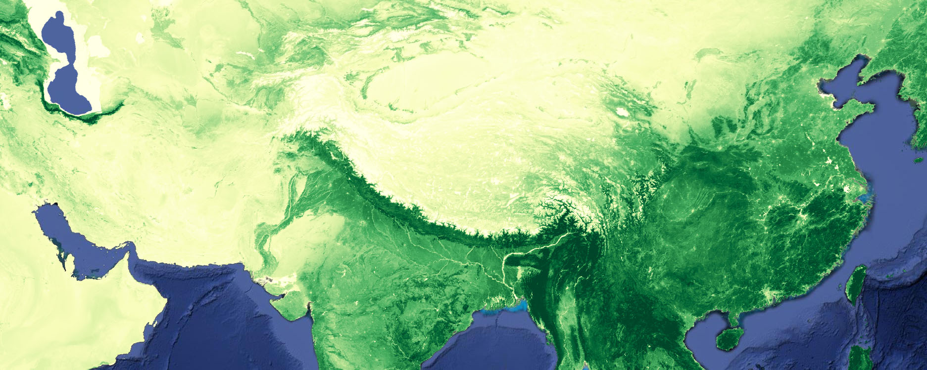
Map.addLayer(grandmean,
{min:0.0, max:0.7, palette:cp.getPalette("YlGn",9)},
'NDVI',1)
Map.addLayer(fit,
{min: -0.006, max: 0.006, bands:'scale', palette: cp.getPalette("PiYG",9)},
'NDVI trends', 0);
Map.addLayer(cor,
{min:-1, max:1, bands:'correlation', palette: cp.getPalette("RdBu",9)},
'Correlation', 0);
Map.addLayer(cor.lte(0.05),
{min: '0', max: '1', bands: 'p-value', palette: ['lightgray','darkgreen']},
'p<=0.05', 0);
// create legends
lg.rampLegend(cp.getPalette("YlGn",9),0,0.7, 'NDVI (-)')
lg.rampLegend(cp.getPalette("PiYG",9), -6e-3,6e-3, 'NDVI trend (y-1)')
lg.rampLegend(cp.getPalette("RdBu",9),-1,1, 'Correlation (-)')
lg.classLegend(undefined, ['False','True'], ['lightgray','darkgreen'], 'Significance')