2 Quality mosaicking
Use a quality mosaicking approach to get both a low tide and high tide image composite, and classify water using simple thresholding on water index to generate a map showing intertidal area.
2.1 Define input data
First we need to define the datasets that we will use. In this exercise you will use Landsat 8 top of atmosphere reflectance data. Copy and paste the lines below to a blank script:
// Settings ======================================
var cloudcov = 20;
var imageQ   = 8;

// get data
var ls8rfl = ee.ImageCollection("LANDSAT/LC08/C01/T1_TOA");
var westerschelde = ee.Geometry.Point(3.83,51.42);

// filter the landsat 8 collection and rename bands
var ls8rfl = ls8rfl
        .filter(ee.Filter.lte('CLOUD_COVER',cloudcov))
        .filter(ee.Filter.gte('IMAGE_QUALITY_OLI',imageQ))
        .map(function(x){
        return x.select(['B2','B3','B4','B5','B6','B10','B7','BQA'])
                .rename(['blue','green','red','nir','swir1','tir','swir2', 'bqa'])
      });
2.2 Mask clouds and calculate index
Often satellite imagery comes with metadata on the quality of the acquired imagery. This can be overall quality indication, such as used above, but also a quality image band, which holds predetermined information on quality of each pixel in the image. Using the cloud and cloud shadow flags in this band, the cloud pixels can be masked for each image in a loop over the image collection.
Because you will need a water index per image in the analysis later on, it is calculated directly in the same loop. The water index that is calculated here is the Normalized Difference Water Index (NDWI), which ranges from -1 (no water) to 1 (water).
// apply cloud mask on per-image basis and add Normalized Difference Water Index band
var util = require('users/philipkraaijenbrink/tools:utilities') // load philip's util functions
var lsmasked = ls8rfl.map(function(x){           // loop over image collection
  var cldmask = util.getQAFlags(x.select('bqa'),4,4,'clouds') // get cloud mask from QA band
  var shdmask = util.getQAFlags(x.select('bqa'),7,8,'shadow') // get cloud shadow mask
  var masked  = x.updateMask(cldmask.eq(0))                   // apply both masks to the image
                .updateMask(shdmask.lte(1))
  var index   = x.normalizedDifference(['green', 'nir'])      // calculate NDWI
                .rename('index')
  var invindex = ee.Image.constant(0).subtract(index) .rename('invindex')// get inverted index
  return masked.addBands(index).addBands(invindex)   // return masked image incl. index bands
})
2.3 Quality mosaic composite
Using the cloud masked imagery, you can now reduce the image collection to two image composites by sorting, on a pixel level, the Landsat images in the collection using the calculated NDWI values. This is performed using qualityMosaic() (see doc), which determines for each pixel in the composite image the image in the collection that has the maximum pixel value for the band specified.
// for each spatial pixel select the image that has the lowest/highest NDWI value
// in the entire (filtered) LS8 image collection
var minwat  = lsmasked.qualityMosaic('invindex');
var maxwat  = lsmasked.qualityMosaic('index');
var meanwat = lsmasked.mean();
Add the data to the map and inspect the results:
2.4 Classify water
Classification of water areas can be performed by applying a threshold on the NDWI values of the image composite. Here, classify the pixels as water when \(\rm{NDWI}>=0.2\). This will create a boolean land-use map with two classes: water = 1, land = 0.
// classify water on both images using NDWI threshold
var lotide = minwat.select('index').gte(0.2);
var hitide = maxwat.select('index').gte(0.2);

// inspect classifications
Map.addLayer(lotide, {palette:['darkgreen','lightblue']}, 'Low tide',true);
Map.addLayer(hitide, {palette:['darkgreen','lightblue']}, 'High tide',true);
Are you satisfied with the classification results?
A better classification can probably be achieved by not selecting the extreme values of the NDWI to generate the image composite (qualityMosaic() function). To do so, a custom index must be constructed than can be passed to qualityMosaic(), for instance one based on percentiles of NDWI.
The function below calculates a low and high NDWI percentile at each pixel based on all images in the filtered image collection. It then determines the difference between the NDWI of each image, at each pixel, with those percentile values. To get the index than can be passed to qualityMosaic(), one takes the absolute of the differences and inverts it, so that the smallest difference becomes the largest value.
// Quite some noise in both classifications because qualitymosaicking picks up the extremes
// Try to improve by using percentiles instead. Percentiles determined by trial and error

// get image with low and high percentile NDWI
var indexperc = lsmasked.select(['index']).reduce(ee.Reducer.percentile([16,99], ['lo','hi']));

// loop over image collection
var lsmasked  = lsmasked.map(function(x){
  // get absolute difference of the percentiles with the NDWI
  var selector = x.select('index').subtract(indexperc).abs();
  // invert to let the min diff be the largest value
  var invsel   = ee.Image.constant(1).divide(selector);
  // add inverted difference band to the image and name properly
  return x.addBands(invsel.rename(['selector_lo','selector_hi']))
});

// use the new selectors to perform the quality mosaic and add to map
var minwat2  = lsmasked.qualityMosaic('selector_lo');
var maxwat2  = lsmasked.qualityMosaic('selector_hi');
Map.addLayer(minwat2, {min:0, max:0.3, bands:['swir1','nir','green']}, 'LT composite v2', true);
Map.addLayer(maxwat2, {min:0, max:0.3, bands:['swir1','nir','green']}, 'HT composite v2', true);
Have a look at the new image composites. This looks much better! They will probably also help to clean up the classification:
// classify water on both images using NDWI threshold
var lotide2 = minwat2.select('index').gte(0.2);
var hitide2 = maxwat2.select('index').gte(0.2);

// inspect classifications
Map.addLayer(lotide2, {palette:['darkgreen','lightblue']}, 'Low tide 2',true);
Map.addLayer(hitide2, {palette:['darkgreen','lightblue']}, 'High tide 2',true);
The intertidal area is than the area that is submerged during high tide (hitide2 = 1), but not submerged during low tide (lotide 2 = 0). Using this Boolean logic, combine both water classifications and subsequently mask out all pixels that are not part of the intertidal area:
// combine with boolean logic to get intertidal area, and mask everything but intertidal
var intertidal = lotide2.eq(0).and(hitide2.eq(1));
var intertidal = intertidal.updateMask(intertidal);

// add to map
Map.addLayer(intertidal, {palette:['red']}, 'Intertidal area',true, 0.75);
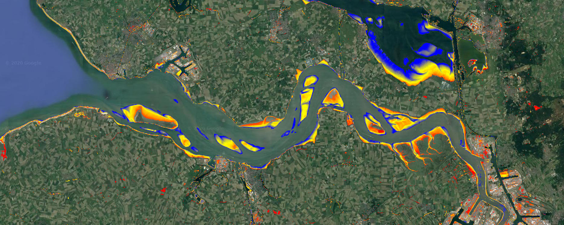
To get a simple proxy for the time that the intertidal beds are submerged during each tide you can use the NDWI value of the mean Landsat composite (average situation):
// use masked mean NDWI of the entire collection to get a proxy for
//the time the intertidal beds are submerged
var subtime = meanwat.select('index').updateMask(intertidal);
var vis_params = {min:-0.1, max:0.4, palette: ['red','yellow','blue']};
Map.addLayer(subtime, vis_params, 'Submerged time', true);
The code works well, with some limitations, for the Western Scheldt estuary. However, Earth Engine allows and advertises with ‘planetary scale analysis’. Visit some other places to see if the code is transferable and scalable (tip: use the search bar as if you were in google maps). For example, check out the Wadden Sea or St. Malo.