4 Climate data analysis
Examine the expected global temperature rise and precipitation changes in the 21st century, aggregate them by country and make a simple global climate change classification.
4.1 Define input data
For this you will use yearly ensemble aggregates of the NEX-GDDP dataset, which is downscaled CMIP5 climate model data. The NEX-GDDP dataset includes daily projections for RCP4.5 and RCP8.5 from 21 Global Circulation Models within CMIP5. The projections include daily minimum temperature, maximum temperature and precipitation for the period 1950–2099. The spatial resolution of the NEX-GDDP dataset is 0.25 degrees (approximately 27 by 27 km at the equator). The original NEX-GDDP data is present in the Earth Engine catalog. For the purpose of this exercise, however, I have pre-aggregated it to yearly data and calculated model ensemble statistics using Google Earth Engine’s computing power.
Load the pre-aggregated NEX-GDDP data, MODIS water mask and custom code:
// load data
var nexy  = ee.ImageCollection('users/philipkraaijenbrink/climate-data/nex-gddp-yearly-stats')
var wmask = ee.Image('MODIS/MOD44W/MOD44W_005_2000_02_24').select('water_mask')

// load custom code
var lg = require('users/philipkraaijenbrink/tools:legends')
var cp = require('users/philipkraaijenbrink/tools:colorpals')
4.2 Estimate mean temperature
Unfortunately, the NEX-GDDP dataset only has minimum and maximum daily temperatures (tasmin, tasmax). For most climate analyses mean daily temperature is used, so you will need to approximate the mean temperature as the average of tasmin and tasmax. Note that this is not accurate and that large deviations are expected, both in space and time. For the purpose of this exercise, however, it will suffice.
// approximate mean temperature above surface for RCP45 and RCP85,
// and store as multiband band image together with precipitation
var start = 2006              // 2006 is start of future for CMIP5
var end   = 2099
var absstack = ee.ImageCollection.fromImages(ee.List.sequence(start,end).map(function(i){
  i = ee.Number(i)
  var curdat = nexy.filterDate(ee.Date.fromYMD(i,1,1),ee.Date.fromYMD(i,12,31))
  var t45  = curdat.filter(ee.Filter.eq('scenario','rcp45')).first()
                    .select(['tasmin_mean','tasmax_mean'])
                    .reduce(ee.Reducer.mean())
                    .rename('tas45')
  var t85  = curdat.filter(ee.Filter.eq('scenario','rcp85')).first()
                    .select(['tasmin_mean','tasmax_mean'])
                    .reduce(ee.Reducer.mean())
                    .rename('tas85')
  var p45  = curdat.filter(ee.Filter.eq('scenario','rcp45')).first()
                    .select(['pr_mean']).rename('pr45')
  var p85  = curdat.filter(ee.Filter.eq('scenario','rcp85')).first()
                    .select(['pr_mean']).rename('pr85')
  var stack  = ee.Image([t45,t85,p45,p85]).set('system:time_start', ee.Date.fromYMD(i,1,1))
  return stack.updateMask(wmask.eq(0))      // limit the analysis to land masses
}))
4.3 Determine relative change
To estimate climate changes that may occur over the course of the 21st century you will need to determine the difference of each year with the climate at the beginning of the century, i.e. the reference climate. It is best practice to determine the difference with a multi-year reference climatology, but for the sake of this exercise you will simply use the first year.
// for each image determine the relative difference with first timestep to get delta T and delta P
var relstack = absstack.map(function(x){
  var baseval  = absstack.filterDate(ee.Date.fromYMD(start,1,1),
                                     ee.Date.fromYMD(start,12,31))
                         .first()
  var deltatas = x.select(["tas45","tas85"])
                  .subtract(baseval.select(["tas45","tas85"]))     // dT (K)
  var deltapr  = x.select(["pr45","pr85"])
                  .subtract(baseval.select(["pr45","pr85"]))
                  .divide(x.select(["pr45","pr85"])).multiply(100) // dP (%)
  return ee.Image([deltatas,deltapr])
           .set('system:time_start', x.get('system:time_start'))
})
4.4 Make charts
You can now create charts of global temperature and precipitation changes relative to 2006 for the two climate scenarios. Add the code below and press run.
// make charts with global average relative climate change for land masses
var glob = ee.Geometry.Polygon([-180,-85,180,-85,180,85,-180,85,-180,-85],
                               'EPSG:4326',
                               false);
var tchart = ui.Chart.image.series(
                 relstack.select(['tas45','tas85']),
                 glob,
                 ee.Reducer.mean(),
                 50000
               )
               .setChartType('LineChart')
               .setOptions({lineWidth: 3, colors: ['6b93ce','af6262']});
var pchart = ui.Chart.image.series(
                 relstack.select(['pr45','pr85']),
                 glob,
                 ee.Reducer.mean(),
                 50000
              )
              .setChartType('LineChart')
              .setOptions({lineWidth: 3, colors: ['6b93ce','af6262']});
print(tchart);
print(pchart);
To show a graph of the absolute mean temperature and precipitation over the period 2006–2099 you could change the data that is plotted by changing relstack to absstack in the above code.
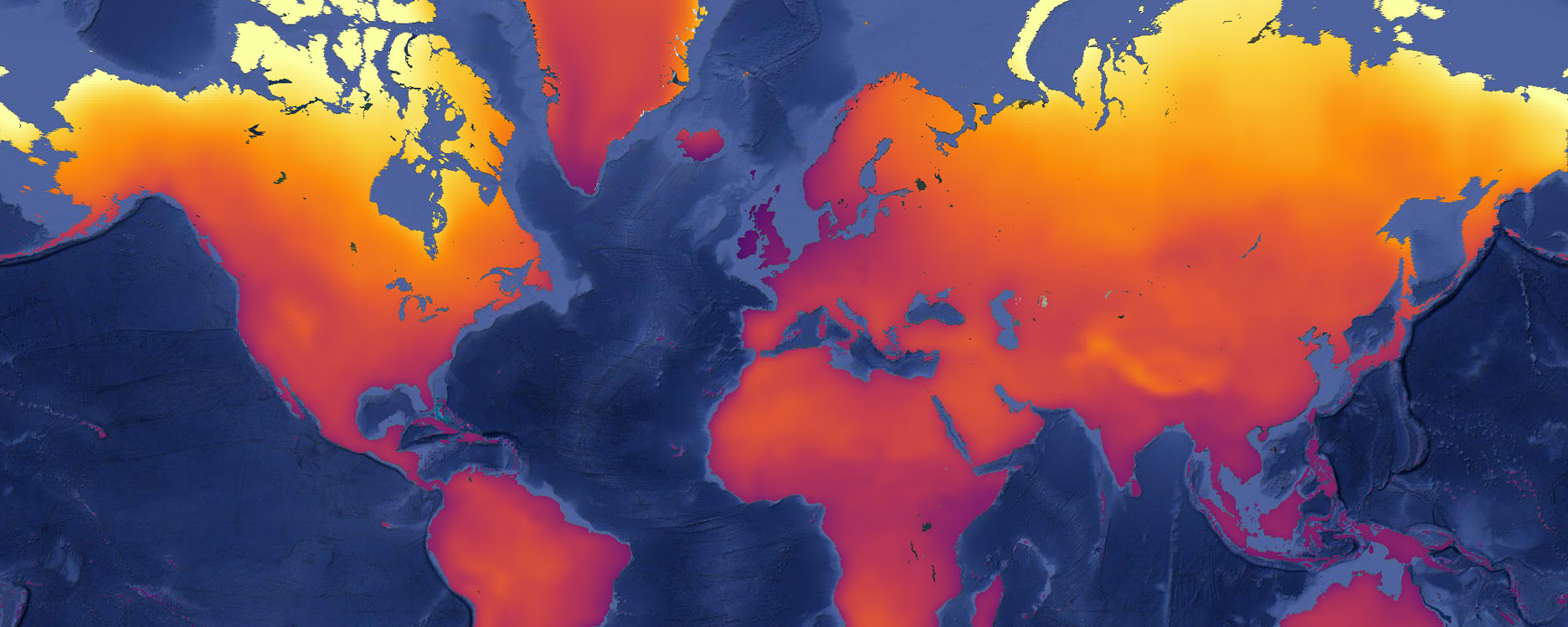
4.5 End of century climatology
Future climate projections are often analysed for specific points in the future instead of transient data. Examples are middle of century (MOC) or end of century (EOC). To limit effects of interannual variability in the data, these points are calculated as climatologies of multiple years. EOC is therefore not just the year 2099, but the mean of 2071–2100.
Calculate the average change in temperature and precipitation for the EOC, add the resulting images for RCP8.5 scenario to the map and inspect the results.
// get end of century (EOC) climatology
var eocmean = relstack.filterDate('2071-01-01','2099-12-31').mean()

// define color palettes to use for tas and pr
var tcol = cp.getPalette('InfernoMPL',9)
var pcol = cp.getPalette('RdBu',5)

// add eoc stats to map
Map.addLayer(eocmean.select("tas85"), {min:0, max:8, palette: tcol}, 'RCP85 dT EOC (K)')
Map.addLayer(eocmean.select("pr85"),  {min:-100, max:100, palette: pcol}, 'RCP85 dP EOC (%)')

// add legends to the map
lg.rampLegend(tcol, 0,8, 'dT EOC (K)')
lg.rampLegend(pcol, -100, 100, 'dP EOC (%)')
To get a sense of climate change impacts in European countries, aggregate the temperature change results by using country polygons. A country dataset is already available in the Earth Engine catalog (Large Scale International Boundaries from the United States Office of the Geographer).
// get warming per country and add to map
var countries = ee.FeatureCollection('USDOS/LSIB_SIMPLE/2017')
countries = countries.filter(ee.Filter.eq('wld_rgn','Europe'))
var countrydeltas = eocmean.reduceRegions(countries,ee.Reducer.mean(),50000)
var dTcountry = ee.Image().float().paint(countrydeltas,'tas85')  // paint poly fill on empty image
var borders   = ee.Image().byte().paint(countries,0,1)   // paint country borders on empty image
Map.addLayer(dTcountry, {min:0, max:8, palette: tcol}, 'dT EOC countries')
Map.addLayer(borders,{},'Country borders')
Finally, make a simple classification of global climate change, given the RCP8.5 scenario. Use four classes: (1) dryer and above average warming, (2) dryer and below average warming, (3) wetter and above average warming, (4) wetter and below average warming.
// make simple end of century classification
var globmean = eocmean.reduceRegion(ee.Reducer.mean(), glob, 50000)   // get global averages for EOC
var dryhot  = eocmean.select('pr85').lt(0)
            .and(eocmean.select('tas85').gte(ee.Image.constant(globmean.get('tas85'))))
var drycold = eocmean.select('pr85').lt(0)
            .and(eocmean.select('tas85').lt(ee.Image.constant(globmean.get('tas85'))))
var wethot  = eocmean.select('pr85').gte(0)
            .and(eocmean.select('tas85').gte(ee.Image.constant(globmean.get('tas85'))))
var wetcold = eocmean.select('pr85').gte(0)
            .and(eocmean.select('tas85').lt(ee.Image.constant(globmean.get('tas85'))))
var classes = ee.Image.constant(0).byte()
            .where(dryhot,0).where(drycold,1).where(wethot,2).where(wetcold,3)
            .updateMask(wmask.eq(0))
var classnames  = ['dryer and relatively hot','dryer and relatively cold',
                'wetter and relatively hot','wetter and relatively cold']
var classcolors = ['#f76754','#f7c054', '#2f6837','#3d8ca0']
Map.addLayer(classes, {min:0,max:3,palette:classcolors}, 'EOC classes')
lg.classLegend(undefined, classnames, classcolors,'EOC classes')